Data Structures & Algorithms Lecture Notes

20 April 2010 • Faster Sorting

---

Outline

• Asymptotically faster sorting.
• A fast O(n²) sort.
• A worst-case O(n log n) sort.
• A worst-case O(n) sort.

Faster Sorting

The previous sorts were all O(n2). Can we do better? How much better can we do?

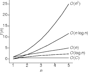
• Remember:

  It's faster only when it's asymptotically faster.

A Question Reasked

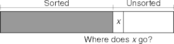
• The question can't be answered until the array's completely sorted.
• Not quite:

  

  • This answer doesn't require sorting.

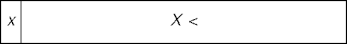
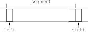
Partitioning

• Partitioning can place x (the pivot):

partition(T a[], int left, int right)
  T pivot = a[left]
  int l = left + 1

  while l < right
    if (a[l] ≤ pivot) l++
    else if (pivot < a[right - 1]) right--
    else swap(a[l++], a[--right])

  swap(a[left], a[--l])
  return l

Quicksort

• Partitioning divides the array into thirds.
  • Repeatedly call partition on the unsorted parts

quicksort(T a[], int left, int right)

  if right > 1 + left
    int mid = partition(a, left, right)
    quicksort(a, left, mid)
    quicksort(a, mid + 1, right)

Quicksort Analysis

• partition() does O(n) work.
• N elements divide in "half" O(log n) times.
  • Each half gets passed to quicksort(), and so to partition().
    • Remember, constants (2 here) don't matter.
• O(log n) iterations, O(n) work per iteration.
  • Quicksort sorts with O(n log n) work.

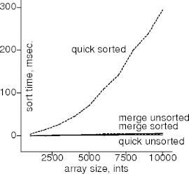
Oh Really?

Well, No

• partition() may not divide into halves.
  • The pivot may be an extreme value.

    

• This has two consequences:
  1. partition() does little useful work.
  2. There are O(n) instead of O(log n) iterations.
     • Quicksort is now O(n²).

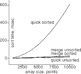
Is It?

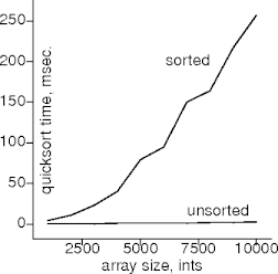
• Worst-case behavior occurs on mostly sorted data.

Avoiding Worst-Case Behavior

• Avoid worst-case quicksort behavior by
  • Not using quicksort on sorted data.
  • Randomly permuting the data.
    • Not too practical.
  • Making a more artful pivot-value choice.

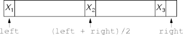
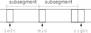
Artful Pivot Choices

• The 3-median pivot value.

  max(min(a[left], a[(left + right)/2])
      min(max(a[left], a[(left + right)/2]), a[right - 1]))
  

• The median-index value.

  a[(left + right)/2]
  

• The random-index value.

  a[left + (rand() mod (right - left))]
  

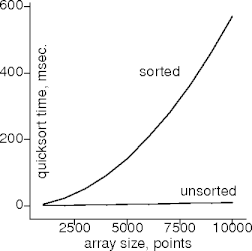
Do They Work?

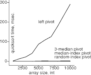
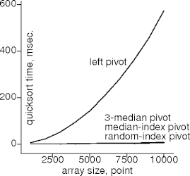
• Worst-case behavior is still O(n²).
  • But it has a low probability of occurrence.

Rigorous Halving

• Quicksort slows down when it can't divide the data evenly.
  • Consistent, even halving results in O(n log n) behavior.
• Is there a sort organized around consistent, even halving?

Divide to Conquer

	Given a data segment,
	divide it into halves.

• Now recurse on the two halves.
  • When do you stop?

Reuniting Divisions

• A segment of size less than two is sorted.
• Two sorted subsegments can be merged back into the original segment.
  • And the original segment will be sorted too.

  

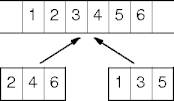
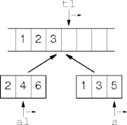
Merging

Scan from left to right, copying the minimum value.

merge(T * tl, tr, al, am, ar) T * s = am while tl < tr if (al < am) ∧ (s == ar or *al < *s) *tl++ = *al++ else *tl++ = *s++

Mergesort

mergesort(T * aleft, aright, tleft, tright)
  int len = aright - aleft
  if len > 1
    int h = len/2
    T * amid = aleft + h
    T * tmid = tleft + h

    mergesort(aleft, amid, tleft, tmid)
    mergesort(amid, aright, tmid, tright)
    merge(
      tleft, tright, aleft, amid, aright)

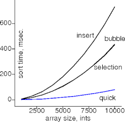
Performance

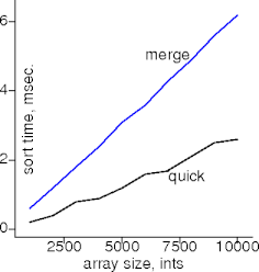
• The extra copying extracts a run-time cost.

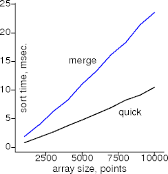
Caveat Emptor

• What does O(n) extra space buy?

• Is it worth it?

Sorting Again

• Remember this?

  

• A heap can answer these questions at a cost of O(log n) per question.
  • That's worst-case O(n log n) total.

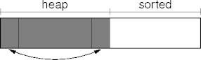
Sorting With A Heap

• Given an array of elements, heapify it.
  • Bubble up successive elements from left to right.
  • This costs O(n log n).
• Remove the max heap element and store it in the open space.

  

Heapsort

heapsort(a[], n)

  for i = 1 to n - 1
    bubble-up(a, i)

  for i = n - 1 to 1
    swap(a[0], a[i])
    bubble-down(i)

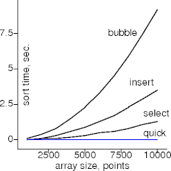
• The constants are worrisome.

Are They?

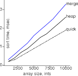
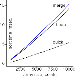
• Apparently.

Some Problems

• AT&T handles about a billion phone calls per day.
  • They all need to be recorded.
  • How do you do it?
• The U.S. Post Office handles about 580 million pieces of mail a day.
  • They all need to be routed.
  • How do you do it?

The Big Idea

• In both cases, the keys are fixed-length numbers.
• A key can be re-interpreted as a base-M number.
  • M is the radix.
  • Two common values are M = 2ⁱ, i > 0, and M = 10.
• The key is decomposed into radix-M digits.

A Radix-10 Example

• To sort a set of three-decimal-digit numbers:
  • Sort the 100s: 000 to 099, 100 to 199, ...
  • Sort each 100s group by 10s: 00 to 09, 10 to 19, ...
  • Sort each 10s group by 1s: 0 to 9.

Radix Exchange Sort

• The previous example with radix-2 digits (binary) is called radix exchange sorting.
• With only two digits, radix exchange sort is similar to quicksort.
  • The partition segregates the ith 0 and 1 bits in the key.

Example Radix Exchange Sort

Radix Exchange Sort

re-sort(int array [], int left, int right, int bit)

  if left + 1 < right and bit < 32
    int mid = partition(array, left, right, bit)
    re-sort(array, left, mid, bit + 1)
    re-sort(array, mid, right, bit + 1)

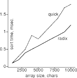
Performance

• Given n b-bit keys, radix exchange sort does
  • O(n) work for each partition, and
  • O(b) partitions.
• Radix exchange sort does O(nb) worst-case work.
  • This is more than O(n) but sometimes less than O(n log n).
  • b is independent of n, but is not constant.

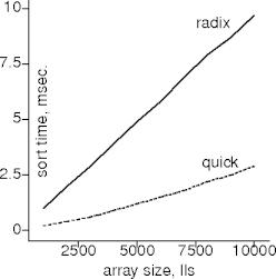
Oh Really?

• When b = 8, b < log₂ n when n = 256, but
  when b = 64, b < log₂ n when n > 1.8×10¹⁹.

The Last Step

• We still don't have a linear sort.
• Let's go back to the mail room. How does a mailroom sort mail?
  • Each recipient has a mailbox.
  • Each piece of mail is placed in the recipient's mailbox.
  • This is a linear-time sort.

Requirements

• A linear-time sort has two requirements:
  1. Enough space to store the sorted values.
  2. A constant-time addressing scheme to locate values in the space.
• A sort meeting these requirements is known as a bucket (or distribution) sort.

Data Structures

• An array meets the linear-sort requirements.
  • Its size is equal to the number of elements being sorted.
  • Indexing is a constant function of the values being sorted.
• Other data structures can also support linear-time searches.

Bucket Sort

• Assume 3-digit decimal numbers.

  bucket_sort(int a[], int n)
  
    int counts[1000]
  
    for i = 1 to n
      counts[a[i] + 1]++
  
    int j = 1
    for i = 1 to 1000
      while counts[i]-- > 0
        a[j++] = i - 1
  
    assert(j == n)
  

References

• Sorting out Sorting (≈30 min) by Ronald Baecker, University of Toronto, 1981 (faster, ≈3 min, but not quiter).
• Algorithm 232: Heapsort by J.W.J Williams, Communications of the ACM, June 1964.

---

This page last modified on 15 April 2010.