Lecture Notes for Simulation
4 April 2005 - Hypothesis Testing
Outline
Answering questions.
Statistical Hypotheses
Hypothesis Testing and Outliers
Accepting vs. Rejecting
Hypotheses
Error types and controlling errors.
One- and two-tailed tests.
Answering Questions
Simulation provide numeric answers.
A mean
m
within bounds
b
at confidence
c
%.
Simulations can also provide yes-no answers.
"Is it worth making this change to the system?"
"Yes (or no) with
s
% significance."
Yes-no answers tend to be of greater interest to decision makers.
Numeric and yes-no answers are essentially similar.
The data and underlying solution methods are identical.
The interpretations differ, as do the solution techniques
Yes-no answers use a statistical-analysis technique known as
hypothesis testing
.
Statistical Hypotheses
A
statistical hypothesis
(or just
hypothesis
) is a predicate over one or more populations.
50% of Monmouth students are between 60 and 72 inches tall.
Server utilization is within 10% of 0.8.
As a predicate, a hypothesis can be considered true or false only when taken over the whole population.
As a practical matter, the truth or falsity of a hypothesis is determined by considering a sample from the related population.
The results of the sample may not be relevant to the population.
A statistical hypothesis does not buy improved accuracy.
However, you may be able to
exploit the analysis to shift priorities
.
Hypothesis Testing and Outliers
Hypothesis testing recognizes and counts outliers in the sample.
Too many outliers is not a good sign.
Is a coin fair if it's flipped fifty times and
it comes up heads twelve times?
it comes up heads thirty times?
The probability of consistently picking outliers from a tailed population is low.
A tailed population probably didn't produce a set of consistent outliers.
Relying on Outliers
Relying on outliers has two consequences:
You can't be sure your outlier determination.
Fifty flips of a fair coin can produce only twelve heads.
But it's highly unlikely.
If they're not outliers, you can't say what they are.
Fifty flips of non-fair coin can result in thirty heads.
And, because you don't know how unfair the coin is, you can't say how unlikely it is.
Accepting vs. Rejecting
A hypothesis may either be
accepted
or
rejected
.
However, because of sampling, accepting and rejecting are not complimentary.
A rejected hypothesis can be considered false.
An accepted hypothesis may or may not be true.
There's not enough evidence reject the hypothesis.
But the evidence to accept isn't conclusive either.
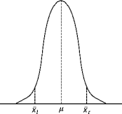
Test Set-Up
Draw
n
samples from a population with mean
m
and variance
v
2
.
Compute
x
; by the Central Limit Theorem,
x
is from an approximately normal distribution with mean
m
and variance
v
2
/
n
.
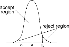
The reject region is known as the
critical area
.
x
l
and
x
r
are known as the
critical values
.
Accept the hypothesis if
x
l
<=
x
<=
x
r
, otherwise reject it.
The critical area and values are parameters to the test.
Hypotheses
Because rejecting's more definitive than accepting, the idea is to accept the hypothesis and try to reject it.
This is the
null hypothesis
, denoted
H
0
.
Given the set-up, the null hypothesis is an equality.
If the null hypothesis isn't rejected, it's not necessarily accepted.
It's just not obviously wrong.
If the null hypothesis is rejected, we can accept the inverse hypothesis.
This is the
alternative hypothesis
, denoted
H
a
.
The alternative hypothesis is an inequality.
Defining the hypotheses can be tricky.
Example Hypotheses
Is the mean server utilization equal to 0.8?
H
0
:
m
= 0.8.
H
a
:
m
!= 0.8.
The interest is in not rejecting the null hypothesis.
Is the mean server utilization greater than than 0.8?
H
0
:
m
= 0.8.
H
a
:
m
> 0.8.
The interest is in rejecting the null hypothesis.
Error Types
A hypothesis test can go wrong by
rejecting a true null hypothesis or
accepting a false null hypothesis.
A
type I error
or a
false negative
rejects a true null hypothesis.
A
type II error
or a
false positive
accepts a false null hypothesis.
Controlling Type I Errors
A type I error (false negative) occurs when a sample rejects
H
0
when it's true.
This occurs when the sample mean exceeds the critical values.
The critical area is the probability of this happening.
It's known as the
significance level
.
False negatives can be controlled by adjusting the critical region or values.
Assuming the critical region or values aren't fixed by the problem.
Type I Error Examples
Is the mean server utilization within 10% of 0.8?
The critical values are
x
l
= 0.8 - 0.08 = 0.72 and
x
r
= 0.88.
Let
v
= 0.1;
z
= (
x
-
m
)/
v
= 0.08/0.1 = 0.8.
From the normal table,
P
(
z
< 0.8) = 0.79.
The critical region is (1 - 0.79)*2 = 0.42.
With a 1 in 10 chance of being wrong, is the mean server utilization 0.8?
P
(
z
0.95
<
z
) = 1.65.
1.65 = (
x
- 0.8)/0.1;
X
= 1.65(0.1) + 0.8 = 0.965.
x
r
= 0.965;
x
l
= 0.8 - 0.165 = 0.635.
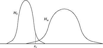
Controlling Type II Errors
A type II error (false positive) occurs when a sample does not reject a false null hypothesis.
False positives depend on the form of the alternative hypothesis.
The probability that
x
is a false positive is
b
=
P
a
(
x
<
x
r
).
The probabilities of type I and II errors are inversely related.
And type I errors are directly controllable.
The false-positive probability decreases as the two distributions separate.
Type II Error Examples
Suppose the server utilization distribution actually has
m
= 0.9 and
v
= 0.01.
The null hypothesis is
m
is within 10% of 0.8.
The critical value is
x
r
= 0.88.
The false-positive probability is
b
=
P
a
(
x
< 0.88).
z
b
= (
x
r
-
m
)/
v
= (0.88 - 0.9)/0.01 = -2
From the normal table,
P
a
(
z
< -2) = 0.02.
There's a 1 in 50 chance of a false positive on the high side.
By symmetry, the chance on both sides is 1 in 25.
One- and Two-Tailed Tests
The null hypothesis specifies distribution parameter equality.
Otherwise, false positives are uncontrollable.
The alternative hypothesis negates the null hypothesis.
The negation of an equality is either an inequality or an ordering.
Given
H
0
:
p
=
p
',
H
a
is either
p
!=
p
',
p
<
p
', or
p
>
p
'.
An alternative hypothesis with inequality results in a
two-tailed hypothesis test
.
The critical region is split symmetrically about the parameter under test.
An alternative hypothesis with ordering results in a
one-tailed hypothesis test
.
The critical region is to the left (
p
<
p
') or right (
p
>
p
') of the parameter under test.
Test Tail Examples
The average wait time is 5 minutes.
The null hypothesis is
H
0
:
m
= 5.
The alternative hypothesis is
H
a
:
m
!= 5.
This is a two-tailed test: a
x
can falsify
H
0
by being too large or too small.
The average wait time does not exceed 5 minutes.
The null hypothesis is
H
0
:
m
= 5.
The alternative hypothesis is
H
a
:
m
> 5.
This is a one-tailed test:
x
can falsify
H
0
only by being too large.
Unknown Population Variance
The variance of the hypothesis population may not (probably won't) be known.
Do the usual trick: substitute the sample variance for the population variance.
For 30 or more samples, the sample mean is still a standard normal distribution.
For
n
< 30 samples, the sample mean is a
t
-distribution with
n
- 1 degrees of freedom.
t
-Distribution Example
A system runs with a 42 widget/min throughput.
A simulation of proposed system changes results in
m
= 50 w/m and
v
= 11.9 (
n
= 12). Should the changes be implemented?
H
0
:
m
= 42;
H
a
:
m
> 42.
m
r
is
t
-distributed with 11 degrees of freedom.
At 5% significance level,
t
r
= 1.796.
At 1% significance level,
t
r
= 2.718.
t
= (
m
-
m
)/(
v
/
n
0.5
) = (50 - 42)/(11.9/3.5) = 2.35
2.35 is in the 5% critical region; reject
H
0
;
m
is greater than 42 (with a 1 in 20 chance of being wrong).
2.35 isn't in the 1% critical region; don't reject
H
0
;
m
isn't that much greater than 42 (with a 1 in 100 chance of being wrong).
Points to Remember
Hypothesis testing answers yes-no questions.
A hypothesis is a predicate about distributions.
This is flexible, but not obviously so.
Errors occur as false negatives or positives (type I or II).
Error control concentrates on false negatives.
This page last modified on 5 April 2005.