Lecture Notes for Simulation

14 March 2005 - Experiment Behavior

Outline

Stochastic Data Collection

• Simulations produce stochastic samples.

  • Successive experimental samples fluctuate unpredictably.

• Stochastic samples introduce conflicting requirements.

  • A single sample or sample set is unrepresentative.

  • Multiple samples or sample sets are uninterpretable.

    • The samples are drawn from an arbitrary, unknown distribution.

• In the concrete, the problem's even worse.

  • The model's behavior under execution influences the samples too.

    • This may not be a problem, but a reflection of the system being modeled.

Stochastic Consiquences

• Some consiquences of stochastic samples:

  • Single experiment runs are not enough.

  • Experimental results require statistical analysis to deal with (quantify) uncertainty.

  • Models should be built and experiments conducted to reduce unhelpful uncertainty.

• Note there are two forms of uncertainty: within the experiment and between experiments.

Sample Behavior

• Consider the average queue lenght in an ATM simulation.

  • The queue-length sample values fluctuate during the expeiment.

• Sample fluctuations can match one of three patterns:

  1. Steady-state behavior.

  2. Transient behavior.

  3. Regenerative behavior.

• In addition, sample sequences may either be finite or (potentially) infinite.

  • These correspond to experiments that either terminate or can run forever.

  • An ATM simulation can run forever; a bank teller simulation terminates.

Steady-State Behavior

• A sample exhibits steady-state behavior when its values fluctuate around a single value.

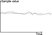
• A sample with steady-state behavior represents stability.

  • Remember, though, that a sample is not the simulation.

• Steady-state sample values have a stable probability distribution.

  • A stable probability distribution is one that doesn't change.

  • In particular, the mean and variance don't change.

• Sample steady-state behavior is the ideal.

  • Flucutations in the steady state are the easiest to handle.

Transient Behavior

• A sample exhibits transient behavior when its values do not fluctuate around a single value.

• A sample with transient behavior represents instability and are essentially unanalyzable.

  • Mercifully, many real systems are generally stable.

  • Experimental systems may not be, and stable systems can exhibit instability.

  • Chaotic systems exhibit permanent instability.

• "Warming-up" instability leads to initial transient behavior.

• It consists of erratic variations that gradually die down in magnitude, leaving the system in a (possibly new) steady state.

Renerative Behavior

• Behavior is said to be regenrative if there exists a particular system state, called a regenerative state, such that whenever the system returns to that state the past history of states of the system has no influence on the future of the system.

  • The point at which the system returns to the regenerative state is called a regenrative (or renewal) point.

• Repeating cycles are seen to start at renerative points were the system parameter is zero, althrough this is not a general requirement.

• A queuing system can be thought of as a regenrativ system if the regeneration points are defined sas those instants when there are no customers in the waiting line and none being served.

Termination

• Typically, each cycle consists of an initial transient period possibly followed by a steady-state period of init duration and then followed by another transient period in which the system returns to the regenerative state.

• A non-terminating system continues indefinitely and the long-term ehavior is usually steady state and therefor predictable.

Transient Effects

• Transient effects can mislead the analyst looking for long-term, steady-state conditions because the system behavior is quite different during transieht and steady-state periods.

  • Ignore the transient state. At this point, all results that have been collected so far are discarded, but the model itself is otherwise unchanged.

  • Pre-load a steady state. One efficient method of assigning an initial state is to use the output of the previous run as the starting conditions for the next run by splitting one long run into a series of shorter subruns connected back to back.

Steady-State Sampling

• An unbiased estimate is one that can be relied upon to converge to the true value as more samples are taken.

• If this process is repeated several times, then we obtain a set of means, each of which has been derived from a different set of samples.

• It seems intuitively reasonable because the mean of the sample meabns is becoming closer and closer to the actual population mean and so the uncertainty of x as expressed by the standard deviation or variance must be decreasing.

The Centeral Limit Theorem

• What is also mathematicall verifiable is that any set of sample means, each of which is calculated from a different set of samples from a fixed, but arbitrary, probability distribution behaves as if it were based on samples from the same probability distribution.

• The Central Limit Theorem:
  If a random sample of size n is taken in the steady state is drawn from a population with fixed mean m and variance v² then the sample mean bar(x) has approximately a normal distribution with mean m and variance v²/n.

• The variance of random samples tends to have less variability than the distribution they come from.
  s² = sum(i = 1, n, (x_i - bar(x))²)

Dealing with Sampling Behavior

• The distinction is made even more important by the fact that a model ordinarily displays several types of behavior, so we must know when each type of behavior starts or becomes dominant and ajdust the treatment accordingly.

Steady-State Detection

• Underestimating the duration of the transient phase introduces unnecessary error, but being too conservative extends the simulation duration more than necessary.

• Additional complexity is added because the transient duration varies with each set of model parameters.

• Transient time duration can be specified in terms of simulated time or else it can be specified in terms of the number of samples to be taken.

• Estimating transient-time duration can be done by monitoring the standard deviation of the sample mean or by calculating a moving average.

Standard-Deviation Monitoring

• Since the Central Limit Theorem applies only when the distribution is stationary, it can be used to test for the onset of the steady state.

• The sample standard deviation is s = s/n^1/2.

• Make the equation linear by taking logs:
  log(s) = log(s) - 0.5 log(n)

  • log(v) is a constant factor and can be ignored.

• In steady state, the graph of log(s) vs. log(n) should be a left-to-right downward diagonal line.

Monitoring The Standard Deviation

• Run the simulation m times, sampling at each run.

  • The sample size n should be around 30 to 50 samples.

• Compute y_i the mean of the i-th sample from each run.
  y_i = sum(j = 1, m, x_ji)/m

• Compute the standard deviation s_n from y_i.
  s_n = (sum(i = 1, n, (y_i - bar(sbs(x, n)))²)/m)^1/2

• Plot lot(s_n) against log(n).

• The value of n when the graph bends properly is the number of samples to skip.

Implementing Standard-Deviation Monitoring

• The step-size parameter defines how many samples are skipped before a value of x_ij is recorded.

• At the end of each individual run the model is reset to the idle state by resetting the random number system, resoures and queues, removing all scheduled and conditional entities, and resetting the clock.

• At the end of the last run the logarithm of the standard deviation is calcualted as a function of the number of samples and printed out.

• The higher utiliztion case also demonstrates the general rule that the higher the utilization the longer it will take to establish steady-state conditions.

Moving Averages

• As each new sample is included the oldest is dropped, thus keeping the number of observations making up the sample constant.

• A method of implementing this approach uses a ring buffer.

• We first subtract the oldest sample from the moving average.

• An alternative approach records all the samples first and when the simulation has finished works out the moving average.

Implementing Moving-Average Monitoring

• Then at the end of each run, with the results accumulated in the array sumx[], the moving average is generated and the results printed.

• A figure of 20 samples when the utilization factor is 4.0 and 100 samples when the utilization factor is 0.6 seems reasonable estimates for the duration of the transient phase based on this evidence.

• It is prudent, therefore, to include a good saftey margin of, say, 50 per cent when the transient duration is estimated.

Points to Remember

This page last modified on 15 March 2005.