1. Let M be an m by n matrix of integers. A chain is a sequence of entries from M starting at M[0, 0] and ending at M[m - 1, n - 1]. If the ith element in the chain is M[i, j], then the (i + 1)th element is either M[i + 1, j] (that is, the entry below M[i, j]), M[i, j + 1] (that is, the entry to the right of M[i, j]) or M[i + 1, j + 1] (that is the entry diagonally below and to the right of M[i, j]):

   

   The sum of a chain is the sum of the matrix entries through which the chain passes.

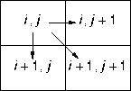
   The problem is to find a chain of maximal sum. Show this problem can be solved using dynamic programming, and develop a dynamic-programming algorithm to solve the problem.

   ---

   Given a chain of maximal sum, divide the chain at any one of the elements M[i, j] through which it passes. The chain from M[0, 0] to M[i, j] must also have maximal sum, otherwise it could be replaced with a chain from M[0, 0] to M[i, j] having a larger sum, contradicting the assertion that the whole chain had a maximal sum. A similar argument shows that the chain from M[i, j] to M[m - also has maximal sum. The optimal-subproblem property holds.

   A recursive solution to this problem follows immediately from the problem statement:

   int max-chain(x, y)
   
     return M[x, y] + max(max-chain(x - 1, y), 
   		       max-chain(x, y - 1),
   		       max-chain(x - 1, y - 1))
   

   Because we're interested in asymptotic behavior, we ignore the boundary conditions. T(n) = 3T(n - 1) is an approximate recurrence relation for max-chain(), where n is the length of the chain; this relation unrolls into an O(n³) and max-chain() has exponential run-time. However, there are only O(mn) maximum sum paths, so the repeated-subproblem property holds.

   Let C be an m by n matrix with C[i, j] equal to the maximal sum of the chain from M[0, 0] to M[i, j]. The dynamic programming solution to the maximal sum chain is

   int max-chain(M)
   
     C[0, 0] <- M[0, 0]
     for i <- 1 to m - 1
       C[0, i] <- C[0, i - 1] + M[0, i]
   
     for i <- 1 to n - 1
       C[i, 0] <- C[i - 1, 0] + [Mi, 0]
   
     for i <- 1 to m - 1
       for j <- 1 to n - 1
         C[i, j] <- M[i, j] + max(C[i - 1, j], 
   		               C[i, j - 1],
   		               C[i - 1, j - 1])
       
     return C[m - 1, n - 1]
   

   max-chain() writes every element of C exactly once, so it's an O(mn) algorithm.

   ---

2. A flow graph is a connected, directed, weighted, acyclic graph with a single node of in-degree zero called the source and a single node of out-degree zero called the sink; for example,

   

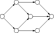
   The problem is to derive an algorithm that finds the minimum cost path from the source to the sink. Show this problem can be solved using dynamic programming, and derive a dynamic programming algorithm that solves the problem.

   ---

   This problem is solved in essentially the same way as was the previous problem; the major difference between the two problems is the way you advance from one subproblem to the next.

   Given a path of minimal cost, divide the path at any one of the nodes n in the path. The subpath from the source to n must also have minimal cost, otherwise it could be replaced with a path from the source to n having a smaller cost, contradicting the assertion that the path had minimal cost. A similar argument shows that the path from n to the sink also has minimal cost. The optimal-subproblem property holds.

   A recursive solution min-path(n), which finds a minimum cost path from the source to node n follows immediately from the problem statement:

   int min-path(n)
   
     m <- infinity
     for each (v, n) in E
       m <- min(m, min-path(v) + w(v, n))
   
     return w
   

   Because we're interested in asymptotic behavior, we ignore the boundary conditions. In the worst case, the approximate recurrence relation for min-path() is T(n) = |E|T(n - 1), where n is the length of the path. This relation unrolls into an O(|E|ⁿ) expression and min-path() has exponential run-time. However, there are only 0(n) minimal paths in the graph, so the repeated-subproblem property holds.

   Let C be an |V|-element vector with C[n] equal to the minimal cost of the path from the source to node n. The dynamic programming solution to the minimal-cost path is

   int min-path(G)
   
     C <- [0, infinity, ..., infinity]
     for x in G.V
       for (u, v) in G.E
         if C[v] > C[u] + w(u, v)
           C[v] <- C[u] + w(u, v)
       
     return C[sink]
   

   This algorithm should look vaguely familiar to you; it's similar to the Bellman-Ford algorithm for single-source shortest paths. Because a flow graph is a DAG, min-path() isn't the most asymptotically efficient algorithm for finding the shortest path; see Section 25.4 of the text for details.

   ---

3. Given a set S of real numbers, the problem is to derive an algorithm that distributes S among a minimal number of sets S₁, ..., S_n such that 1.0 >= max(S_i) - min(S_i); that is, the difference between the largest and smallest element in each subset is no more than one. Show this problem can be solved by greed, and develop a greedy algorithm to solve the problem.

   ---

   Given an minimal solution S₁, ... S_n, order them by increasing maximal element and divide the sets into two parts. The left part must use a minimum of sets to cover the points within the left part; if it didn't, the points could be covered by a smaller number of sets, contradicting the claim that the entire set cover is minimal. A similar argument holds for the right part. The optimal-subproblem property holds.

   The key to a greedy algorithm for the set cover problem is to sort the point set in increasing order (in this case; decreasing order would work too):

   min-set-cover(S)
   
     S <- sort(S)
     covers <- [{}, {}, ..., {}]
     c <- 0
     first <- S[0]
     for i <- 0 to |S| - 1
       if S[i] - first > 1.0
         c++
         first <- S[i]
       covers[c] <- union(covers[c], { S[i] })
       
     return covers
   

   covers is an array of sets covering the input set S. min-set-cover() keeps stuffing points in S into a set in covers until the next point from S is more than 1 away from the smallest element in the current cover set in covers. In that case, min-set-cover() moves on to the next empty cover set in covers, remembers the next point from S as the new smallest element, and continues.

   To show min-set-cover() is correct, we need to show the greedy-choice property holds. Let S₁, ..., S_n be an arbitrary minimal cover for the point set S ordered in increasing order by minimum point. Let s₁ be the smallest point in S and let s₂ be the largest point in S that is no more than 1.0 away from s₂; that is, the greedy algorithm puts points s₁ through s₂ into its first cover set.

   s₁ is in S₁; if any of the other greedy points in s₁ through s₂ are not in S₁, they can be moved into S₁. Note that the set from which the point moved must contain other points not in S₁, otherwise the covering S₁, ... S_n would not be minimal.

   S₁ cannot contain any other points then those in s₁ through s₂ because all other points are more than 1.0 away from s₁. By possibly shifting points among the sets S_i, it is possible to make S₁ equal to the first greedy cover set without changing the number of cover sets. We can now throw away S₁ and the points s₁ through s₂ and repeat the argument. In this way, it's possible to transform any minimal solution to the cover set problem for S into the greedy solution, and the greedy-choice property holds.

   ---

4. Given a list of words w₁, ..., w_n and a function f(i) which indicates the frequency with which word w_i will be looked up, the problem is to construct a binary search tree B which minimizes the comparisons it takes to look up words in the list. Show this problem can be solved with a greedy algorithm, and develop a greedy algorithm to solve the problem.

   ---

   You all should recognize this problem; it's just Huffman's encoding without the encoding part. A binary tree storing the words to minimize comparisons during look up will put the more frequently accessed words nearer the root; more precisely, the binary tree should minimize

   sum(i = 1 to n, d(w_i)f(i))

   The opt-bst() algorithm creates such a tree:

   opt-bst(W, f)
   
     Q <- init(W, f)
     for i <- 1 to |W| - 1
       x <- extract-min(Q)
       y <- extract-min(Q)
       insert(Q, node(x, y, x.f + y.f))
       
     return extract-min(Q)
   

   The proof of the greedy-choice property is as it was for Huffman's algorithm: take an arbitrary optimal tree T and form tree T' by swapping the greedy choices b and c for the maximum depth leaves x and y in T. Then the weights of the two trees are equivalent and the argument continues.

   The proof of the optimal-subproblem property is also as it was for Huffman's algorithm: starting with a greedy optimal tree and create a modified tree by compressing two leaf nodes into a combined leaf node. The resulting tree is also optimal.

   You can find the details on either of these proofs in Section 17.3 of the text.

   ---

This page last modified on 26 April 2000.