BFS'(G, s)

  for each u in G.V - {s}
    color[u] <- white
    distance[u] <- infinity
    parent[u] <- nil

  color[s] <- gray
  distance[s] <- 0
  parent[s] <- nil
  S <- {s}

  while S != { }
    u <- pick(S)
    for each v in neighbor[u]
      if color[v] = white
        color[v] <- gray
        distance[v] <- distance[u] + 1
        parent[v] <- u
        add(S, v)
    color[u] <- black
    remove(S, u)
Is the algorithm BFS'() correct as defined by Theorem 23.4? Justify your answer.
The unreachable v argument doesn't depend on a queue, so it is still valid for BFS'(). The reachable v argument does depend on the queue, and that's where the problem occurs.
The reachable v argument is an inductive argument over Vk, the set of vertices at distance k from the start vertex s. For the argument to be valid, the algorithm must process all vertices in Vk before processing any vertex from Vk + 1. Becuase BFS() uses a queue to store vertices, they are processed in the proper order. However, vertices stored in a set are removed in arbitrary order, and it's possible that BFS'() could process a grandchild before all the children are processed. The result of this misordering could cause errors in the distance vector entries for the greatgrandchildren of the misordered vertices.
For example, consider the graph
Starting at s, BFS() would dequeue the vertices in the order s, u, v (or the reverse), x, and w. Because v is processed before w, v reaches x before w does, and
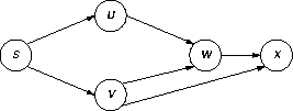
d[x] is correctly set to 2.
BFS'(), on the other hand, can remove vertices from the set in the order
s, u, w, x, and v. In this order w reaches
x before v does, and d[x] gets incorrectly set to 3.
The idea of a cut doesn't change, and neither does the idea of a cut respecting the spanning tree. A light edge isn't helpful, but a heavy edge is: a heavy edge is a cut crossing the edge with a weight greater than or equal to the weight of any edge crossing the cut.
Theorem 24.1 has to be modified to show that a heavy edge for a cut respecting the spanning tree is safe for the spanning tree. For some respecting cut, let the edge (u, v) instead of the heavy edge (x, y) be added to the MST T. Form spanning tree T' by adding (x, y) to T and removing (u, v) from T. Because (x, y) and (u, v) are from the same cut, and (x, y) is a heavy edge, w(x, y) >= w(u, v), and w(T') >= w(T). However, T is a MST, and so w(T') <= w(T), which means that w(T') = w(T) and T' is also a MST. (x, y) is safe for the spanning tree for the same reasons given in Theorem 24.1 as that argument doesn't involve edge weights.
The cost of part set i, 1 <= i <= n is given by the function cost(i). In addition, there is an assembly cost associated with each part set, which depends the number of part sets that have already been added to the chassis; for example, it may be cheaper to add part set i to the chassis first than to add it to the chassis fifth. The function assembly(i, j) gives the cost of adding part set 1 <= i <= n to the chassis when 0 <= j < n part sets have already been added.
The final cost to the customer is the cost of the chassis plus the sum of the costs of the part set picked plus the sum of assembly costs; the customer does not specify an assembly order. To insure speedy service both in calculating the customers' bills and in assembling their cars, you have been given the job of 1) precomputing all possible cars that might be ordered and 2) determining the cheapest way to assemble each car. Your solution to 1) should be a graph and your solution to 2) should be the result of running a graph algorithm over the graph you created to solve 1). How the graph looks and the graph algorithm to use is for you to decide.
Before solving a problem, it is often helpful to examine the problem to determine some of its characteristics, which we might be able to exploit when creating a solution. In this problem, because it asks us to model something by a graph, it might be helpful to know about the number of items to be represented in the graph.
Given n parts from which to choose, each car created will either have or not have part i, which means that there are a total of 2n different cars that can be created. This means that representing each part by a graph vertex won't work: a graph with n vertices can have at most n2 edges (as an upper bound), and n + n2 is less than 2n when n > 4.
Each vertex could represent a particular sequence of assembly for some subset of parts and edges between vertices could represent the "cheaper than" relation between vertices, but that would require computing the cost of each possible assembly, which is the unknown for this problem.
With parts and part sequence eliminated, the only thing left is the cars. Let G be the directed, weighted graph (V, E, W) defined as follows:
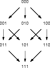
V: The vertices of G are the set of n-bit binary numbers. each number is interpreted as a car with parts; if bit i is 1, the car has part i, if bit i is 0, the car doesn't have part i. For example, with n = 3, the vertex 010 represents the car with part 2 and no other parts; the vertex 000 represent the chassis.For example, the graph for three parts isE: Two vertices of G are connected by an edge if and only if the two vertices differ by exactly one bit; the directed edge goes from the vertex with the zero bit to the vertex with the one bit. For example, with n = 3, there would be a directed edge from the vertex 000 to the vertex 001; there would not be a directed edge from vertex 000 to vertex 011; there would, however, be a directed edge from 001 to 011.
W: The weight of the edge (u, v) is cost(i) + assembly(i, j), where i is the number of the part being installed and j is the number of parts already installed. For example, the edge from 000 to 010 would have weight cost(2) + assembly(2, 0).
(I have omitted the edge weights because I couldn't figure out how to get the graph drawing program to include them properly.)
With the graph G in hand, the solution to the second part of the problem is straightforward: run the single source, all destinations shortest path algorithm over G with the chassis vertex as the source. The shortest path from the chassis vertex to some other vertex v describes the assembly order that gives the cheapest cost to build the car described by v.
Your colleague's observation is correct: the gray vertex color is not needed to do a proper depth-first search. The DFS-Search algorithm must avoid visiting a vertex more than once, and for that a boolean value (or black and white) is enough.
Your colleague's recommendation is not useful, however. While three colors are not necessary, the algorithm depends on white and gray, and deleting line 1 would break DFS-Visit(). To see why, consider running DFS() with the modified DFS-Visit() on the graph
With line 1 deleted, DFS-Visit() will infinitely recurse because both the vertices u and v will be always be white.

To be useful, you colleague's recommendation should have been to delete line 7 in DFS-Visit().