Becuase a polynomial reduction only does a polynomial amout of work (or, equivelently, works for a polynomial amount of time), it can only affect a polynomial change on the input string, and so the size of the output string will be a polynomial factor of the input string.
The Hamiltonian cycle problem accepts a graph and returns true if there exists a simple cycle that passes through all vertices in the graph exactly once. The TSP problem accepts a weighted, complete graph and an integer itl(k) and returns true if there is a simple cycle through the graph and the weight of the cycle is at most itl(k), where the weight of a cycle is the sum of the weights of the edges making up the cycle.
The reduction from the Hamiltonian cycle problem to the TSP takes an instance of the Hamiltonian cycle problem and constructs an instance of the TSP as follows:
- take the graph itl(G) associated with the Hamiltonian cycle problem and form the weighted graph itl(G)' by copying itl(G) and assigning a weight of 1 to each edge in itl(G)'.
- turn itl(G)' into a complete weighted graph by including an edge between every pair of vertices in itl(G)' that do not have an edge in itl(G). Assign a weight of |itl(V)| + 1, where itl(V) is the set of vertices in itl(G)' (or itl(G)), to the new edges.
- assign |itl(V)| to itl(k).
This reduction is polynomial in the number of vertices in the original graph itl(G).
Now to show the reduction preserves correctness. Let itl(H) be an instance of the Hamailtonian cycle problem and the TSP instance itl(T) be the reduction of itl(H). Assume itl(H) returns true; that is, the given graph contains a Hamiltonian cycle. Then the same cycle serves as a TSP cycle for the graph in itl(T) and the weight of the cycle is at most itl(k), so itl(T) also returns true. Now assume itl(T) returns true; then there exists a simple cycle of weight at most itl(k) = |itl(V)|. Because each of the edges added to itl(G)' but not in itl(G) have weight |itl(V)| + 1, none of the new edges are part of the cycle, and the cycle also serves as the Hamiltonian cycle for the graph in itl(H); itl(H) also returns true. Because the reduction maps solutions to solutions on both sides of the reduction, it preserves correctness.
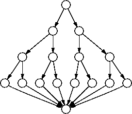
The key to solving this problem is to recognize that the set of all paths between two nodes in a graph has exponential size. For example, consider the total number of paths between the entry and exit nodes in the program graph
Because the set of paths has exponential size, any algorithm that generates the set must do an exponential amount of work, and so cannot be in NP. For example (and remember, examples are not proofs), consider an NP algorithm using correct choice:
  s <- { }
  while (p <- choice(G)) != nil
    s <- union(s, {p})
nil if no such path exists. The while loop iteration
count is bounded by an exponential, so the whole algorithm has exponential
running time (this analysis is sloppy because I'm ignoring potentially
exponential work when dealing with the set itl(s); however because I account
for exponential work in the iteration bound, it is still, more or less,
correct).
The knapsack decision problem accepts as input a set itl(X) of elements, an integer size itl(S), and an integer value itl(V). Each element itl(x) of itl(X) has associated with it a size itl(size)(itl(x)) and a value itl(value)(itl(x)). The knapsack decision problem produces as output true if there exists a subset itl(K) of itl(X) such that the sum of the sizes of the elements in itl(K) are at most itl(S) and the sum of the values of the elements in itl(K) are at least itl(V) and false if no such subset exists.
The knapsack algorithm must generate subsets of the itl(X), examining each subset to see if it's suitable in terms of itl(S) and itl(V), and backtrack to the next subset if the current subset isn't suitable. Perhaps the easiest way to generate subsets is to consider each element of itl(X) in turn. Assuming element itl(x) of set itl(X) is part of an acceptable subset, the knapsack algorithm recurses to find a suitable subset of itl(X) - {itl(x)}. If it can't find such a subset, it must backtrack to the incorrect assumption that itl(x) is part of the subset and try again, this time without adding itl(x) to the subset. If the algorithm still can't find a suitable subset, there is no such acceptable subset in itl(X).
bool knapsack(X, current_s, current_v)

  if X == {}
    return current_s <= total_s and total_v <= current_v

  x <- an element of X

  if knapsack(X - {x}, current_s + size(x), current_v + value(x))
    return true

  if knapsack(X - {x}, current_s, current_v)
    return true

  return false
knapsack(). Letting itl(T)(itl(n))
be time it takes knapsack() to execute on an itl(n)-element set, the two
if statments take
itl(T)(itl(n) - 1) + itl(T)(itl(n) - 1) = 2*itl(T)(itl(n) - 1)time to execute (note that itl(T)() represents the exact solution to
knapsack()'s behavior, and with exact solutions constants do matter; it
would be incorrect to omit the constant 2). Working through the recurrence
relation shows that itl(T)(itl(n)) = 2itl(n), and that overall
knapsack() has Theta(2itl(n)) worst-case behavior.
We can do a little branch-and-bounding to try and improve knapsack()'s
average-case behavior by replacing the first if statement with
if current_s > total_s
  return false

if X == {}
  return total_v <= current_v