You should present your algorithms in enough detail to convincingly argue their correctness. You may use the same type of node in each algorithm; child-sibling form will use just two of the itl(k) available pointers in the node (you may also assume itl(k) > 1).
To start, define the type tree-node as
type tree-node = record {
  data     : T
  children : array [1..k] of pointer to tree-node
  }
k > 1. If the tree node t is being used in a child-sibling
tree, t.children[1] is the pointer to t's children, and
t.children[2] is a pointer to the first of t's siblings; the other
values in the children array are undefined. If t is being used in a
itl(k)-child tree, the pointers to t's children may appear anywhere in
t.children when t has less than itl(k) children.
The key point to exploit when designing the transformation algorithms is that trees are recursive data structures. We can save ourselves a lot of work by designing recursive algorithms to match the structure of the trees. To get some idea of the amount of work you can save, compare the recursive implementation of DFS shown in Figure 7.4 of the text to the non-recursive implementation shown in Figure 7.8 (although I think most of that extra work is a result of the author's unusual placement of postWORK in the DFS algorithm).
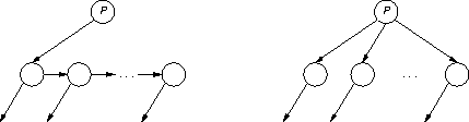
The following diagram shows what happens when a node itl(P) is translated from child-sibling form (which I'll call binary from now on) to k-child form:
Although simple, this diagram does show one subtle point: node itl(P) in its binary form doesn't have a sibling pointer (this not the same thing as saying that itl(P) doesn't have any siblings - if itl(P) had no siblings, it would still have a nil sibling pointer). This is an important point, because if itl(P) had a sibling pointer at the start of the conversion, it would get clobbered as pointers to itl(P)'s children are added to itl(P). One useful way to think about this point is that, even though itl(P) is not yet in itl(k)-child form, it's part of a k-child tree; itl(P)'s siblings are being pointed to directly by itl(P)'s parent, and itl(P)'s sibling pointer is no longer needed.
With these points in mind, the conversion algorithm follows directly:
 void binary2k(P: tree-node)

  children <- P.children[1]
  i <- 1

  do children != nil
    P.children[i] <- children
    children <- children.children[2]
    binary2k(P.children[i])
    i <- i + 1
  od
binary2k() follows down the sibling chain of itl(P)'s children, adding a
copy of each sibling pointer to itl(P) as a child pointer. Once each sibling
has been linked to itl(P) as a child, it is part of a tree in itl(k)-child form
and may be safely used as an argument to a recursive binary2k() call.
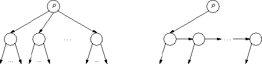
The next diagram shows a k-child to binary conversion:
This diagram makes a point similar to that made by the previous diagram, but this time it's not so subtle: itl(P)'s children have to be in binary form before itl(P) is converted to binary form. If itl(P)'s children were not in binary form, then storing the sibling pointer in a child might clobber pointers to the child's children.
void k2binary(P: tree-node)

  siblings: tree-node
  child: pointer to tree-node

  siblings.children[2] <- nil

  do i <- k to 1 by -1
    child <- P.children[i]
    if child != nil
      k2binary(child)
      child.children[2] <- siblings.children[2]
      siblings.children[2] <- child
    fi
  od

  P.children[1] <- siblings.children[2]
k2binary() uses a dummy record called siblings to simplify how the
sibling list is formed; this trick is described on page 66 of the text. The
sibling list is created from the end to the start, so searching through the
children backwards preserves the left-to-right order of the children
(binary2k() also preserves left-to-right order). Each of itl(P)'s
children is recursively passed to k2binary() to make sure the sibling link
in the child doesn't contain a pointer to a child of the child.
Unfortunately, the text is correct. The AVL property is a global property: it must hold throughout the AVL tree. The difference in heights between itl(B)'s subtrees in Figure 4.13a is at most one, but the difference in heights between itl(A)'s subtrees - that is between subtrees itl(B) and itl(C) - is more than 1, and the tree must be rebalanced.
One way to solve this problem is to have two auxiliary arrays the same size as the input array. The algorithm copies the even elements to one auxiliary array, the odd elements to the other auxiliary array, and then copies the contents of the auxiliary arrays back into the input array in the proper order. This algorithm is obviously correct, but it copies the data 2itl(n) times, where itl(n) is the size of the input array, and requires 2itl(n) extra space. Is there another, more efficient algorithm?
With respect to copying data, note that even elements at the left end of the input array don't have to be moved; they're already in place. Similarly, odd elements at the right end of the input array can be left alone. With respect to auxiliary storage, an odd element in the left end of the input array can be swapped with an even element in the right end, which requires one temporary variable.
These observations suggest an algorithm that sweeps through the array. There would be two sweeps through the array, one from each end, sweeping towards the other end of the array. The sweeps stop when they meet somewhere in the array. Each sweep advances when it discovers a new element of the proper parity (even or odd) and swaps elements with the other sweep when they discover elements of the wrong parity. The algorithm is
void eo-sort(a)

  l <- 0
  r <- |a|

  invariant: a[1..l] is even and a[r + 1..|a|] is odd and l <= r

  do l < r
    if a[l + 1] is even then l <- l + 1
    or a[r] is odd then r <- r - 1
    or a[l + 1] is odd and a[r] is even then
       a[l + 1] <-> a[r]
       l <- l + 1
       r <- r - 1
    fi
  od
a.
The first two statements of eo-sort() establish the invariant. There are no
elements in either a[1..0] or a[|a| + 1..|a|], so the even-odd
requirements are trivially true. Note that the index l points to the
right end of the even numbers in a, but the index r points to the
element (if any) adjacent to the left end of the odd numbers in a:

The first two branches of the if statement advance each sweep if the element
adjacent to, but not part of, the sweep has correct parity; each of these
branches maintains the invariant. The third branch of the if statement performs
the swap when the each sweep is adjacent to elements of the wrong parity
(<-> is the swap operator).
The do statement terminates because each iteration reduces r - l, the
value of which can't go below zero because of the invariant l <= r. When
the do statement terminates, l < r is false; that is l >= r is true.
From this and the invariant it must be that l = r. This lets us conclude
that all elements in a[1..l] are even, that all elements in a[l +
1..|a|] are odd, and that eo-sort() is correct.
eo-sort() makes no unnecessary data movements because a swap is performed
only when an even element is found to the right of an odd element in the array,
and it uses the minimum amount of temporary storage to perform the swap
(ignoring exclusive-or tricks). Any algorithm without special knowledge about
the input array most test the parity of every element in the array, so
eo-sort() is an efficient algorithm.
Let the array a represent one list and the array b represent the
other list. One approach is to systematically compare each item in a to
all items in b:
i <- 1
do i <= |a|
  j <- 1
  do j <= |b|
    if a[i] = b[j] then return true
    j <- j + 1
  od
  i <- i + 1
od
return false
a and b - this approach
makes O(|a||b|) comparisons (in fact, it makes exactly
|a||b| comparisons).
This approach makes no use of the fact that a and b are sorted. How
can that knowledge be exploited? One observation to make is that if b[j]
is greater than a[i], there is no need to consider further elements of
b because they would be at least as large as b[j], and so would also be
greater than a[i]. This observation leads to the modified approach
i <- 1
do i <= |a|
  j <- 1
  do j <= |b|
    if a[i] = b[j] then return true
    or a[i] < b[j] then break
    fi
    j <- j + 1
  od
  i <- i + 1
od
return false
a||b|) (consider the case when there are no
matches and the last element of a is greater than the first element of
b).
The expensive worst case behavior occurs because of nested loops. Is there
another observation available to help get rid of one of the loops? A little
thought shows that if a[i] < b[j], it must be the case that
a[i] > b[1..j-1] because otherwise the comparison between a[i] and
b[j] would never have occurred. Because a is sorted in ascending
order, a[i] <= a[i+1], and it follows that a[i+1] > b[1..j-1]
too. This means that, when increasing i, it is not necessary to reset
j to 1, and the search can continue were it left off in b. These two
observations lead to the code
A loop iteration either terminates the search or advances the search through one element of the input lists. The worst case behavior is now O(|a| + |b|). In the absence of other knowledge about the input arrays, each element in either array needs to be compared to at least one element of the other array, so this code is efficient.i <- 1 j <- 1 do i <= |a| and j <= |b| if a[i] = b[j] then return true or a[i] > b[j] then j <- j + 1 or a[i] < b[j] then i <- i + 1 fi od return false